Example Q4: Running a Basic Experiment

This example notebook shows how run Auspex qubit experiments using the fake data interface.

© Raytheon BBN Technologies 2018

First we ask auspex to run in dummy mode, which avoids loading instrument drivers.

import auspex.config as config
config.auspex_dummy_mode = True

from QGL import *
from auspex.qubit import *
import matplotlib.pyplot as plt
%matplotlib inline

Channel library setup

cl = ChannelLibrary(":memory:")
pl = PipelineManager()

q1 = cl.new_qubit("q1")
aps2_1 = cl.new_APS2("BBNAPSa", address="192.168.2.4", trigger_interval=200e-6)
aps2_2 = cl.new_APS2("BBNAPSb", address="192.168.2.2")
dig_1  = cl.new_X6("Dig_1", address="1", sampling_rate=500e6, record_length=1024)
h1 = cl.new_source("Holz_1", "HolzworthHS9000", "HS9004A-009-1", reference='10MHz', power=-30)
h2 = cl.new_source("Holz_2", "HolzworthHS9000", "HS9004A-009-2", reference='10MHz', power=-30)

cl.set_measure(q1, aps2_1, dig_1.ch(1), trig_channel=aps2_1.ch("m2"), gate=False, generator=h1)
cl.set_control(q1, aps2_2, generator=h2)
cl.set_master(aps2_1, aps2_1.ch("m1"))
cl["q1"].measure_chan.frequency = 0e6
cl["q1"].measure_chan.autodyne_freq = 10e6

auspex-INFO: 2019-04-04 17:36:36,136 ----> Could not find an existing pipeline. Please create one.

Pipeline setup

pl.create_default_pipeline()

pl["q1"].stream_type = "raw"
pl.recreate_pipeline(buffers=False)
pl.show_pipeline()

pl["q1"]["Demodulate"]["Integrate"]["Average"].add(Display(label="Plot Average", plot_dims=1), connector_out="partial_average")
pl["q1"]["Demodulate"]["Integrate"].add(Display(label="Plot Integrate", plot_dims=1))
pl.show_pipeline()

Initialize software demodulation parameters. If these are not properly configured than the Channelizer filter will report ‘insufficient decimation’ or other errors. The integration boxcar parameters are then defined.

demod = pl["q1"]["Demodulate"]
demod.frequency = cl["q1"].measure_chan.frequency
demod.decimation_factor = 16

integ = pl["q1"]["Demodulate"]["Integrate"]
integ.box_car_start = 0.2e-6
integ.box_car_stop= 1.9e-6

Taking Fake Data

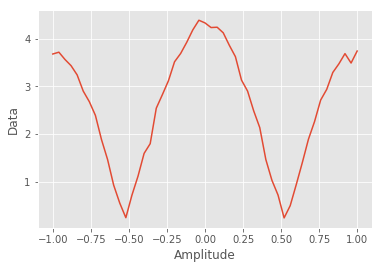
Now we create a simple experiment, but ask the digitizer to emit fake data of our choosing. This is useful for debugging one’s configuration without having access to hardware. The set_fake_data method loads the fake dataset into the indicated digitizer’s driver. The digitizer driver automatically chooses the nature of it’s output depending on whether receiver channels are raw, demodulated, or integrated.

amps = np.linspace(-1,1,51)
exp = QubitExperiment(RabiAmp(q1,amps),averages=50)
exp.set_fake_data(dig_1, np.cos(np.linspace(0, 2*np.pi,51)))
exp.run_sweeps()

Compiled 51 sequences.
Qubit('q1') has 1

auspex-INFO: 2019-04-04 17:38:10,603 ----> Connection established to plot server.

Plotting the Results in the Notebook

exp.get_final_plots()

Loading the Data Files and Plot Manually

data, desc = exp.outputs_by_qubit["q1"][0].get_data()

plt.plot(desc["amplitude"], np.abs(data))
plt.xlabel("Amplitude"); plt.ylabel("Data");

Plotting and the Plot Server & Client

The Display nodes in the filter pipeline are turned into live plotters. In the auspex/utils directory once can find auspex-plot-server.py and auspex-plot-client.py. The server, which should be executed first, acts as a data router and can accept multiple clients (and even multiple concurrent Auspex runs). The client polls the server to see whether any plots are available. If so, it grabs their descriptions and constructs a tab for each Display filter. The plots are updated as new data becomes available, and will look something like this:

For every execution of run_sweeps on an experiment, a new plot will be opened. In the plot client menus, however, the user can close all previous plots as well as choose to ‘Auto Close Plots’, which closes any previous plots before opening another.

Remote Usage

The plot server and client can be run remotely, as can the Jupyter notebooks one expects to run. By running the following ssh port-forwarding command:

ssh -R 7761:localhost:7761 -R 7762:localhost:7762 -L 8889:my.host.com:8888 -l username my.host.com

You could connect to a remotely running Jupyter notebook on port 8888 locally at port 8889, and then (after starting auspex-plot-server.py and auspex-plot-client.py on your local machine) watch new plots appear in a live window on your local machine.

This presumes one does not have unfettered network access to the remote host, in which case ssh tunneling is not necessary. Currently the plotter and client assume they are all connecting on localhost, but we will create a convenient interface for their configuration soon.

Monitoring Changes in the Channel Library

The session keeps track of what values have changed without being committed, e.g.:

cl.session.commit()
cl.session.dirty

Everything is in sync with the database. Now we modify some property:

aps2_1.ch(1).amp_factor = 0.95
cl.session.dirty

We see that things have changed that haven’t been committed to the database. This can be rectified with another commit, or optionally a rollback!

cl.session.rollback()
aps2_1.ch(1).amp_factor